8 Values and Means
The concept of value is expressible in the metric units by which the character is measured. The value observed when the character is measured on an individual is the phenotypic value of that individual. All observations, whether of means, variances, or covariances, must clearly be based on measurements of phenotypic values.
The first division of phenotypic value is into components attributable to the influence of genotype and environment. The genotype is the particular assemblage of genes possessed by the individual, and the environment is all the non-genetic circumstances that influence the phenotypic value.
\[P = G + E\]
where P is the phenotypic value, G is the genotypic value, and E is the environmental deviation.
The mean environmental deviation in the population as a whole is taken to be zero, so that the mean phenotypic value is equal to the mean genotypic value. The term population mean then refers equally to phenotypic or to genotypic values.
For the purposes of deduction we must assign arbitrary values to the genotypes under discussion. Considering a single locus with two alleles, \(A_1\) and \(A_2\), we cal the genotypic value of one homozygote +a, that of the other homozygote -a and that of the heterozygote d. (we shall adopt the convention that \(A_1\) is the allele that increases the value).

Fig. 7.1. Arbitrarily assigned genotypic values
8.1 Population mean
Table 7.1
| Genotype | Frequency | Value | Freq. * Val. |
|---|---|---|---|
| \(A_1A_1\) | \(p^2\) | +a | \(p^2a\) |
| \(A_1A_2\) | 2pq | d | 2pqd |
| \(A_2A_2\) | \(q^2\) | -a | -q^2a |
| Sum = | a(p-q)+2pqd |
The population mean is thus
\[M = a(p-q)+2dpq\]
This is both the mean genotypic value and the mean phenotypic value of the population with respect to the character. The contribution of any locus to the population mean thus has two terms: a(p-q) attributable to homozygotes, and 2dpq attributable to heterozygotes. If there is no dominance (d=0), M = a(1-2q); if ther is complete domiance (d=a), \(M = a(1-2q^2)\). The total range of value attributable to the locus is 2a, in the abseence of overdomiance. (M=-a when q=1; M=a when q=0)
We suppose that the combination of genes at several loci is by addition. Then the population mean:
\[M = \sum a(p-q) + 2\sum dpq\]
8.2 Average effect
The value associated with genes(alleles) as distinct from genotypes is known as the average effect.
There are several ways in which average effects can be defined. One defination is this: the average effect of a particular gene (allele) is the mean deviation from the population mean of individuals which received that gene (allele) from one parent, the gene (allele) from the other parent havving come at random from the population.
Table 7.2
| Type of gamete | genotype \(A_1A_1\) (a) | genotype \(A_1A_2\) (d) | genotype \(A_2A_2\) (-a) | Mean value of genotypes produced | Population mean to be deducted | Average effect of gene(allele) |
|---|---|---|---|---|---|---|
| \(A_1\) | p | q | pa+qd | a(p-q)+2dpq | q(a+d(q-p)) | |
| \(A_2\) | p | q | -qa+pd | - | -p(a+d(q-p)) |
The gametes carring \(A_1\) unite at random with gametes from the population, the frequencies of the genotypes will be p of \(A_1A_1\) and q of \(A_1A_2\). The genotypic value of \(A_1A_1\) is +a and that of \(A_1A_2\) is d, the mean is pa+qd. The difference between this mean and the population mean is the average effect of the gene (allele) \(A_1\), which we use the symbol \(\alpha_1\):
\[\alpha_1 = pa+qd-(a(p-q)+2dpq) = q(a+d(q-p))\]
Similarly, the average effect of the gene \(A_2\) is
\[\alpha_2 = -p(a+d(q-p))\]
The average effect of the gene substitution (allele substitution) is simple the difference between the average effects of two alleles:
\[\alpha = \alpha_1 - \alpha_2 = a + d(q-p)\]
And then the average effects of the two alleles, when expressed in terms of the average effect of the gene substitution, are
\[\alpha_1 = q\alpha\]
\[\alpha_2 = -p \alpha\]
8.3 Breeding value
The value of an individual, judged by the mean value of its progeny, is called the breeding value of the individual.
For a single locus with two alleles, the breeding values of the genotypes are as follows:
| Genotype | Breeding value |
|---|---|
| \(A_1A_1\) | \(2\alpha_1 = 2q\alpha\) |
| \(A_1A_2\) | \(\alpha_1 + \alpha_2 = (q-p)\alpha\) |
| \(A_2A_2\) | \(2\alpha_2 = -2p\alpha\) |
Consideration of the definition of breeding value will show that in a population in HWE the mean breeding value must be zero.
\[2q\alpha \times p^2 + (q-p)\alpha \times 2pq -2p\alpha \times q^2 = 2pq\alpha(p+q-p-q)=0\]
8.4 Dominance deviation
For a single locus, the difference between the genotypic value G and the breeding value of A of a particular genotype is known as the dominance deviation D, so that
\[G = A + D\]
## initial the value
a = 1
d=3/4
q=1/4
## calculate other values
p=1-q
population_mean = a*(p-q) + 2*d*p*q  ### population mean
alpha = a + d*(q-p)                  ### the average effect of an allelic substitution
alpha1 = q*alpha                     ### average effect of A1 allele
alpha2 = -p*alpha                    ### average effect of A2 allele
## vectors
genotype = c(0,1,2)                  ### genotype coded by the number of allele A1
genotype_value = c(-a,d,a)           ### gennotypic values
genotype_frq = c(q^2, 2*p*q, p^2)    ### genotype frequence
breeding_value = c(-2*p*alpha,(q-p)*alpha, 2*q*alpha)      ### breeding values for each genotype group
## plot - basic frame
par(mar = c(5,4,4,4) + 0.1)
plot(c(0,2),c(-1.2,1.2),col="white",xaxt="n",yaxt="n",xlab="Frequency",ylab="Genotypic values")
mtext("Breeding values", side = 4, line = 3, cex = par("cex.lab"))
axis(side=2, at=c(genotype_value,0), labels= c("-a","d","+a","0"),las=1)
axis(side=1, at=c(0,1,2),labels=c("A2A2(0)","A1A2(1)","A1A1(2)"))
axis(side = 4, at=c(breeding_value,0)+population_mean, labels= c("-2pα","(q-p)α","2qα","0"),las=1)   ### Breeding value is deviations from the population mean.
## plot - genotypic values
points(genotype, genotype_value,pch=16)
## plot - the regression line, Fisher's decomposition
y = rep(genotype_value,genotype_frq*16)
x = rep(genotype, genotype_frq*16)
lmfit = lm(y~x)
b0 = lmfit$"coeff"[1]
b1 = lmfit$"coeff"[2]
abline(b0,b1)
## plot - some indicating lines, points
points(0,population_mean+2*alpha2)
points(1,population_mean+alpha1+alpha2)
points(2,population_mean+2*alpha1)
lines(c(0,1),c(population_mean+2*alpha2,population_mean+2*alpha2),lty=2)
lines(c(1,1),c(population_mean+2*alpha2,population_mean+alpha1+alpha2),lty=2)
text(0.5,population_mean+2*alpha2+0.1,"1")
text(1.05,population_mean+2*alpha2+0.3,"α")
lines(c(0,0),c(-a,population_mean+2*alpha2),lty=3)
lines(c(1,1),c(population_mean+alpha2+alpha1,d),lty=3)
lines(c(2,2),c(a,population_mean+2*alpha1),lty=3)
points((population_mean-b0)/b1,population_mean, pch=3)  ### population mean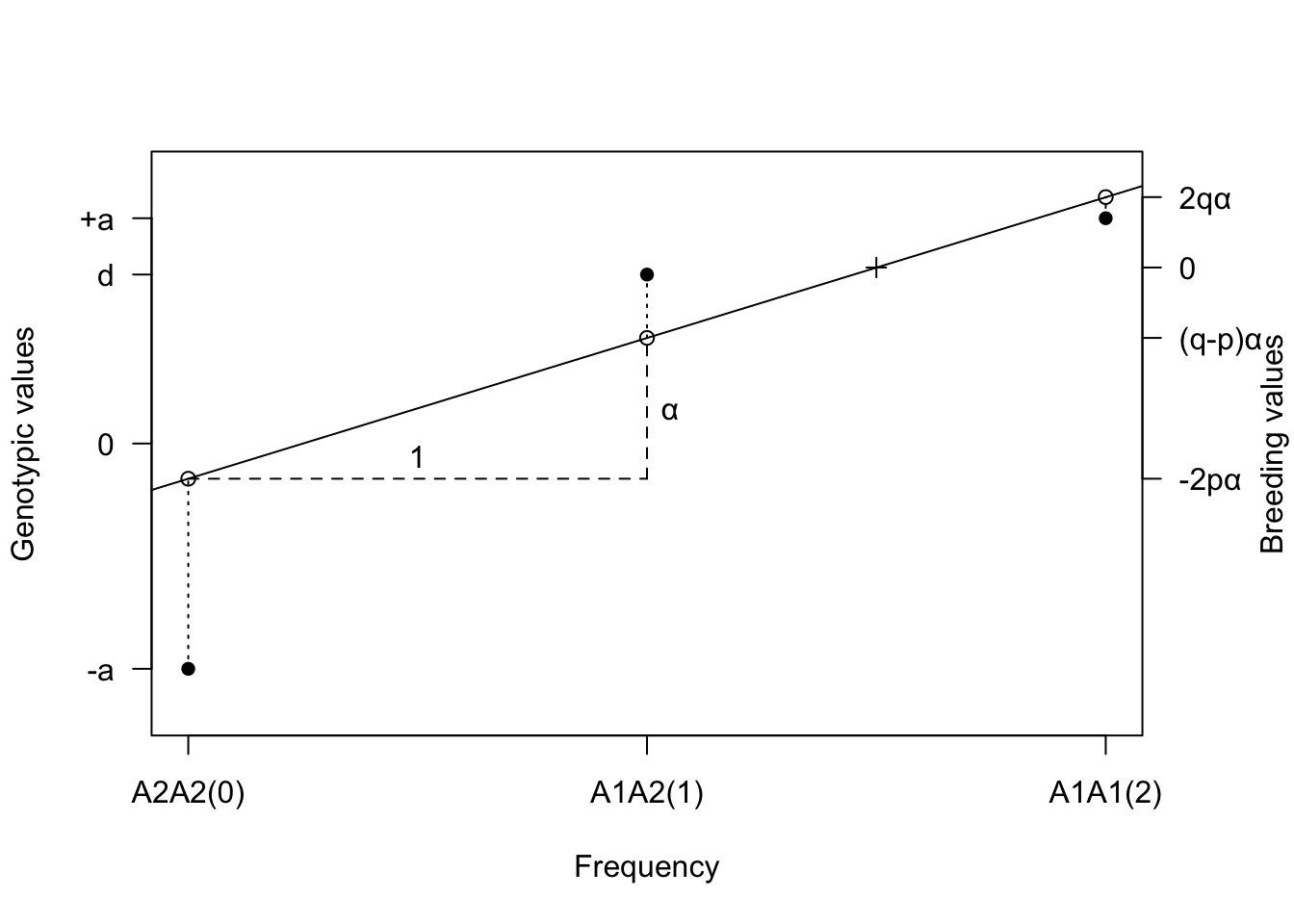
In the figure,
- The genotypic values (closed circles) are plotted against the number of \(A_1\) genes in the genotype
- A straight regression line is fitted by least squares to these points, each point being weighted by the frequency of the genotype it represents.
- The position of this line gives the breeding values of each genotype, as shown by the open circles.
- The differences between the breeding values and the genotypic values are the dominance deviations (D), indicated by vertical dotted lines.
- The cross marks the population mean.
- The average effect \(\alpha\) of the gene substitution is given by the difference in breeding value between \(A_2A_2\) and \(A_1A_2\), or between \(A_1A_2\) and \(A_1A_1\) as indicated.
Note: Bruce Walsh's slides are good supplement resouces.
Table 7.3 Values of genotypes in a two-allele system, measured as deviations from the population mean.
- Population mean: M = a(p-q)+2dpq
- Average effect of gene substitution: \(\alpha\) = a+d(q-p)
| Genotype | \(A_1A_1\) | \(A_1A_2\) | \(A_2A_2\) |
|---|---|---|---|
| Frequencies | \(p^2\) | \(2pq\) | \(q^2\) |
| Assigned values | a | d | -a |
| Genotypic value\(^a\) | \(2q(a-pd)\) | \(a(q-p)+d(1-2pq)\) | \(-2p(a+qd)\) |
| Genotypic value\(^b\) | \(2q(\alpha-qd)\) | \((q-p)\alpha+2pqd\) | \(-2p(\alpha+pd)\) |
| Breeding value | \(2q\alpha = 2\alpha_1\) | \((q-p)\alpha=\alpha_1+\alpha_2\) | \(-2p\alpha=2\alpha_2\) |
| Domiance deviation | \(-2q^2d\) | \(2pqd\) | \(-2p^2d\) |
- The genotypic value is deviations from population mean and in terms of a
- The genotypic value is deviations from population mean and in terms of \(\alpha\)
From the table above, if there is no domiance, d is zero and the domiance deviations are also zero. Therefore in the absence of dominance, breeding values and genotypic values are the same. Genes that show no domiance (d=0) are sometimes called "additive genes", or are said to "act additively".
8.5 Interaction deviation
When the genotype refers to more than one locus, the genotypic value may contain an additional deviation due to non-additive combination. Let \(G_A\) be the genotypic value of an individual attributable to one locus, \(G_B\) that attributable to a second locus, and G the aggregate genotypic value attributable to both loci together. Then
\[G = G_A + G_B + I_{AB}\]
where \(I_{AB}\) is the deviation from additive combination of these genotypic values.
If I is not zero for any combination of genes at different loci, those genes are said to "interact" or to exhibit "epistasis", the term epistasis being given a wider meaning in quantitative genetics than in Mendelian genetics. The deviation I is called the interaction deviation or epistatic deviation.
For all loci together we can write,
\[G = A + D +I\]
where A is the sum of the breeding values attributable to the separate loci, and D is the sum of the dominance deviations.
8.6 Note: Proof of the slope of regression line
| genotype | allele A1 number(x) | genotypic value(y) | frequency |
|---|---|---|---|
| \(A_1A_1\) | 2 | +a | \(p^2\) |
| \(A_1A_2\) | 1 | d | \(2pq\) |
| \(A_2A_2\) | 0 | -a | \(q^2\) |
\(E(x) = 2p^2 + 1 \times 2pq + 0 \times q^2 = 2p\)
\(Var(x) = 2pq\)
\(E(y) = a \times p^2 + d\times 2pq + (-a)\times q^2 = a(p-q)+2dpq \text{ (Population mean)}\)
\(E(xy) = 2 \times a \times p^2 + 1 \times d \times 2pq + 0 \times (-a) \times q^2 = 2pqd + 2ap^2\)
\(Cov(y,x)= E(xy) - E(x)E(y) = 2pqd+2ap^2-2p\times (a(p-q)+2dpq) = 2pq(d(q-p)+a)\)
\(b_1 = \frac{Cov(y,x)}{Var(x)} = d(q-p)+a = \alpha\)