GWAS simulation setting

update at 19/Jan/2024

I revisit this post after reading Section 4.4 in the book Casella and Berger, Statistical Inference (2001)

===================

Simulation is a common method to study (bio)statistics, like quantitavie genetics or gwas (genome-wide association study).

A common way to simulate a phenotype based on one simulated SNP (e.g. Wu et al. Genome Biology 2017) is:

y = g + e; g = wu

y is a simulated phenotype
w is a simulated standardized (mean 0 and variance 1) genotype, calculated by w = (x-2f)/sqrt(2f(1-f))
- x is a simulated genotype, generated from Bin(2, f)
- f is the minor allele frequency, generated from Uni(0.1, 0.5)
u is the effect size per standardized genotype, generated from N(0,1)
g is the genetic value, calculated by wu
e is the error term, generated from N(0, var(g)(1/h2 - 1))
h2 is the variance explained by the genotype (heritability)

Constant value vs random variable

In this setting,

y, w, x, and e are random variables
h2 is a parameter, which is usually set manually

Importantly note that

f and u are also constant values, although it is generated randomly

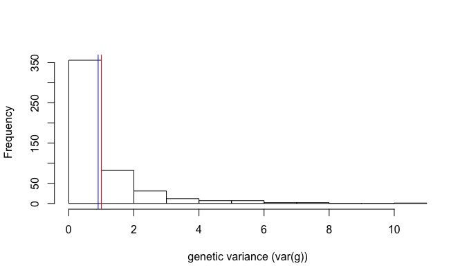
var(g) = var(wu) = u^2var(w) = u^2

E(var(gu)) = E(u^2) = var(u) + E(u)^2 = 1 + 0^2 = 1

R code

We can verify the above in R

set.seed(7)
n=10000; rep=500; res=c()
for(repindex in 1:rep){
    f = runif(1, 0.1, 0.5)
    x = rbinom(n, 2, f)
    w = (x-2*f)/sqrt(2*f*(1-f))
    u = rnorm(1)
    g = w*u
    res = c(res, var(g))
}
hist(res, main = "", xlab="genetic variance (var(g))") ### emprical distribution
abline(v=1, col="red")   ### expected value
abline(v=mean(res), col="blue")  ### emprical value