sampling distribution of correlation r
two independent variables
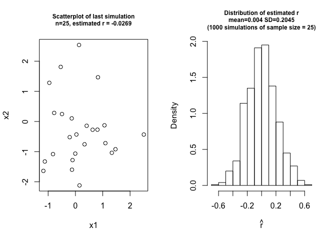
If r is the correlation coefficient of two independent variables x1 and x2, then r should be 0. However the sample estimation of r is not exactly 0. There is a sampling distribution around 0.
rep = 1000; n = 25
set.seed(1)
cors = c()
for(i in 1:rep){
  x1 = rnorm(n)
  x2 = rnorm(n)
  r = cor(x1,x2)
  cors = c(cors, r)
}
layout(matrix(1:2,1,2))
par(cex.main=0.75)
plot(x1, x2, main = paste("Scatterplot of last simulation\nn=",n,", estimated r = ", round(r,4), sep=""))
hist(cors, main = paste("Distribution of estimated r\nmean=",round(mean(cors),4)," SD=",round(sd(cors),4),"\n(",rep," simulations of sample size = ",n,")", sep=""), xlab=expression(hat(r)), freq=F)
two correlated variables
However, if the population correlation is not equal to 0, the distribution of estimated r is skewed.
rep = 1000; n = 25
set.seed(1)
cors = c()
for(i in 1:rep){
  x1 = rnorm(n)
  x2 = rnorm(n)
  r = cor(x1,x1+2*x2)
  cors = c(cors, r)
}
layout(matrix(1:2,1,2))
par(cex.main=0.75)
plot(x1, x2, main = paste("Scatterplot of last simulation\nn=",n,", estimated r = ", round(r,4), sep=""))
hist(cors, main = paste("Distribution of estimated r\nmean=",round(mean(cors),4)," SD=",round(sd(cors),4),"\n(",rep," simulations of sample size = ",n,")", sep=""), xlab=expression(hat(r)), freq=F)
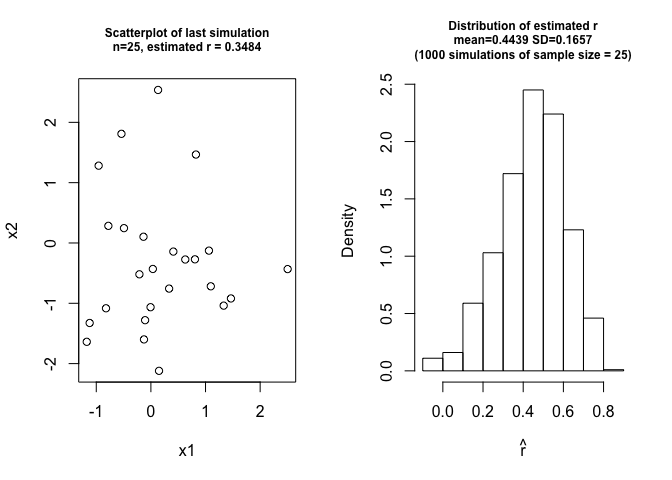
Note that if x1 and x2 are two independent standard normal variables, the correlation between x1 and x1+2*x2 should be:
\[cor(x_1,x_1+2x_2) = \frac{cov(x_1, x_1+2x_2)}{\sqrt{var(x_1) \times var(x_1+2x_2)}}\] \[= \frac{cov(x_1,x_1)+2cov(x_1,x_2)}{\sqrt{var(x1)\times (var(x_1)+4var(x_2)+2\times 2 \times cov(x_1,x_2))}}\] \[= \frac{1+0}{\sqrt{1 \times 5}} = 0.4472136\]Fisher’s z transformtion
Fisher developed a way to r to z’:
\[z' = \frac{1}{2} \times ln\frac{1+r}{1-r} \sim N( \mu, \frac{1}{\sqrt{N-3}} )\]rep = 1000; n = 25
set.seed(1)
zs = c()
for(i in 1:rep){
x1 = rnorm(n)
x2 = rnorm(n)
r = cor(x1,x1+2*x2)
z = log((1+r)/(1-r))/2
zs = c(zs, z)
}
layout(matrix(1:2,1,2))
par(cex.main=0.75)
plot(x1, x2, main = paste("Scatterplot of last simulation\nn=",n,", estimated r = ", round(r,4),", z' = ", round(z,4), sep=""))
hist(zs, main = paste("Distribution of z'\nmean=",round(mean(zs),4)," SD=",round(sd(zs),4),"\n(",rep," simulations of sample size = ",n,")", sep=""), xlab="z'", freq=F)
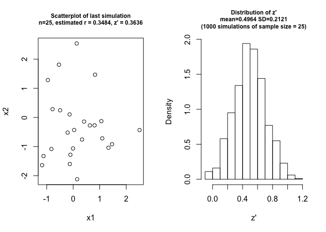
### The mean of z'
0.5 * log((1+0.4472136)/(1-0.4472136))

## [1] 0.4812118

### The standard error of z'
1/sqrt(n-3)

## [1] 0.2132007