HWE and LD

Hardy-Weinberg equilibrium and Linkage disequilibrium are two basic concepts in population genetics.

Defination

Hardy-Weinberg Equilibrium (HWE): allele and genotype frequencies in a population will remain constant from generation to generation in the absence of other evolutionary influences.
Linkage Disequilibrium (LD): the non-random association of alleles at different loci in a given population.

So HWE is about the allele and genotype frequencies in one locus, but LD is about alleles at different loci.

Hardy-Weinberg Equilibrium

From Genotype to Allele frequencies

For $n_{AA}, n_{Aa}, n_{aa}$ is the count of genotype AA, Aa and aa, respectively. And $n = n_{AA} + n_{Aa} + n_{aa}$.

So, the count of A and a alleles are:

\[n_{A} = 2 \times n_{AA} + n_{Aa}\] \[n_{a} = 2 \times n_{aa} + n_{Aa}\]

The frequencies of A and a alleles are:

\[p_{A} = \frac{n_{A}}{2n} = \frac{2 \times n_{AA} + n_{Aa}}{2n} = p_{AA} + \frac{1}{2}p_{Aa}\] \[p_{a} = \frac{n_{a}}{2n} = \frac{2 \times n_{aa} + n_{Aa}}{2n} = p_{aa} + \frac{1}{2}p_{Aa}\] \[p_{A} = 1 - p_{a}\]

From Allele to Genotype frequencies - HWE

We cannot directly get genotype frequencies from allele frequencies. But under Hardy-Weiberge Equilibrium, we can do it by

\[p_{AA} = p_{A}^{2}\] \[p_{Aa} = 2p_{A}p_{a}\] \[p_{aa} = p_{a}^{2}\]

The assumptions for HWE includes:

random mating
infinite population size (no genetic drift)
no mutation
no selection
no migration

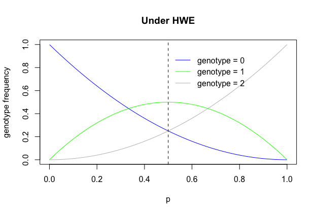
In addition, we can see genotype frequencies is a binomial distribution. If SNP genotpes are coded X = 0, 1 and 2 (alleles) and the allele frequency is p, then:

\[X \sim B(2, p)\text{ with }E(X) = 2p\text{ and }Var(X)=2p(1-p)\]

We can plot the distribution of three different genotypes. In real genetics, we usually use the minor allele, so p is less than 0.5.

p = seq(0,1,0.01)
plot(p, (1-p)^2, ylab = "genotype frequency", main="Under HWE",type="l", col="blue")
lines(p, 2*p*(1-p), col="green")
lines(p, p^2, col="grey")
legend(0.5,0.95,"genotype = 0",lty = 1, col ="blue", bty="n")
legend(0.5,0.85,"genotype = 1",lty = 1, col ="green", bty = "n")
legend(0.5,0.75,"genotype = 2",lty = 1, col ="grey", bty = "n")
abline(v = 0.5, lty=2)

Test for HWE

In the GWAS QC step, we usually remove SNPs with extensive deviation from HWE because this can be indicative of a genotyping or genotype-calling error.

The two common ways to test HWE are Chi-square test and exact test.

For Chi-square test:

\[\chi^{2} = \frac{(n_{AA}-e{AA})^2}{e_{AA}} + \frac{(n_{Aa}-e{Aa})^2}{e_{Aa}} + \frac{(n_{aa}-e{aa})^2}{e_{aa}}\]

where $e_{AA} = np_{A}^2$, $e_{Aa} = 2np_{A}p_{a}$, $e_{aa} = np_{a}^2$ and df = 1 (#genotype - #allele).

For exact test:

\[P(N_{Aa}|N_{A}) = \frac{n_{A}!n_{a}!n!2^{n_{Aa}}}{\frac{1}{2}(n_{A}-n_{Aa})!n_{Aa}!\frac{1}{2}(n_{a}-n_{Aa})!(2n)!}\]

For example, a sample with 2504 individuals, the observed genotypes are 2467/36/1 for AA, Aa and aa. We can do the chi-square test in R.

### Observed genotype counts
n_AA = 2467
n_Aa = 36
n_aa = 1
n = n_AA + n_Aa + n_aa
O_geno = c(n_AA, n_Aa, n_aa)
cat(O_geno)

## 2467 36 1

### Observed allele count and frequency
n_A = n_AA * 2 + n_Aa
n_a = n_aa * 2 + n_Aa
p_A = n_A/(2 * n)
p_a = n_a/(2 * n)
cat(p_A, p_a)

## 0.9924121 0.007587859

### Expected genotype count, under HWE
E_AA = p_A^2 * n
E_Aa = 2 * p_A * p_a *  n
E_aa = p_a^2 * n
E_geno = c(E_AA, E_Aa, E_aa)
cat(E_geno)

## 2466.144 37.71166 0.1441693

### Chi-square with df=1 (#genotypes - #alleles)
chisq = sum((O_geno-E_geno)^2/E_geno)
pvalue = 1 - pchisq(chisq, 1)
cat(paste("chisq:", chisq, ";","pvalue: ", pvalue))

## chisq: 5.15844350552391 ; pvalue:  0.02313362043297

We can also use the R package “HardyWeinberg” to do the chi-square test.

### We can also use the R package "HardyWeinberg"
library(HardyWeinberg)
HWChisq(O_geno, cc=0)

## Chi-square test for Hardy-Weinberg equilibrium (autosomal)
## Chi2 =  5.158444 DF =  1 p-value =  0.02313362 D =  -0.8558307 f =  0.04538812

It’s hard to do the exact test directly in R because of the factorial calucation. So we also use the R package “HardyWeinberg”. A more common way is to use PLINK “–hwe” option.

HWExact(O_geno)

## Haldane Exact test for Hardy-Weinberg equilibrium (autosomal)
## using SELOME p-value
## sample counts: n =  2467 n =  36 n =  1 
## H0: HWE (D==0), H1: D <> 0 
## D =  -0.8558307 p-value =  0.1318891

We can see that the p-values from chi-square and exact test are quite different. In 2005, Wigginton et al has shown that the chi-square inflated type I error rates. So exact test is a better method.

Linkage disequilibrium

Disequilibrium coefficient (D)

For a pair of biallelic loci, there are four haplotypes. If there is no association between these two SNPs (linkage equilibrium), the haplotype frequencies should be:

$p_{AB} = p_{A} \times p_{B}$
$p_{aB} = p_{a} \times p_{B}$
$p_{Ab} = p_{A} \times p_{b}$
$p_{ab} = p_{a} \times p_{b}$

However, if the two SNPs have nonrandom association, the LD can be defined by disequilibrium coefficient:

$D_{AB} = p_{AB} - p_{A} \times p_{B}$
$P_{AB} = p_{A} \times p_{B} + D_{AB}$
$p_{aB} = p_{a} \times p_{B} - D_{AB}$
$p_{Ab} = p_{A} \times p_{b} - D_{AB}$
$p_{ab} = p_{a} \times p_{b} + D_{AB}$

Other LD measures

More wildely used measures for LD are D’ (LEWONTIN 1964) and $r^{2}$ (HILL and ROBERTSON 1968).

\[D'_{AB} = \frac{D_{AB}}{D_{min}}\] \[D_{min} = max(-p_{A}p_{B}, -p_{a}p_{b}), if D_{AB} < 0\] \[D_{min} = min(p_{A}p_{b}, p_{a}p_{B}), if D_{AB} > 0\]

D′ = 1 indicates that at least one of the four possible haplotypes is absent, regardless of the allele frequencies.

\[r^{2} = \frac{D^{2}}{p_{A}p_{a}p_{B}p_{b}}\]

$r^{2}$ is a correlation coefficient of 1/0 (all or none) indicator variables indicating the presence of A and B.

Influence Factor

Linkage disequilibrium is influenced by many factors, including,

selection
the rate of recombination
the rate of mutation
genetic drift
the system of mating
population structure
genetic linkage.

An example in R

Haplotype table

haplotype	ab	Ab	aB	AB
frequency	0	32/5008	1/5008	4975/5008

2*2 allele frequency table

allele	a	A	Total
b	0	32/5008	32/5008
B	1/5008	4975/5008	4976/5008
Total	1/5008	5007/5008	1

#haplotype frequency
pab = 0
pAb = 32/5008
paB = 1/5008
pAB = 4975/5008
cat(pab, pAb, paB, pAB)

## 0 0.006389776 0.0001996805 0.9934105

#allele frequency
pa = paB + pab
pA = pAB + pAb
pb = pab + pAb
pB = paB + pAB
cat(pa, pA, pb, pB)

## 0.0001996805 0.9998003 0.006389776 0.9936102

#D
D = pAB - pA*pB
cat(D)

## -1.275914e-06

#Dmin
Dmin = max(-pA*pB, -pa*pb)
cat(Dmin)

## -1.275914e-06

#D'
Ddot = D/Dmin
cat(Ddot)

## 1

#r-square
rsq = D^2/(pa*pA*pb*pB)
cat(rsq)

## 1.284376e-06