Simple Statistic in R
After reading all the materials of one Statistic Mooc, I would like to use R to practice these statistic equations.
Descriptive Statistics
sample mean
\[\bar{x} = \frac{1}{n}\displaystyle\sum_{i=1}^{n}x_{i}\]x = 1:10
mean(x)
## [1] 5.5
sample variance, standard deviation
\[Var(x) = \frac{1}{n-1}\displaystyle\sum_{i=1}^{n}(x_{i} - \bar{x})^{2}\] \[Var(x) = \frac{1}{n-1}(\displaystyle\sum_{i=1}^{n}x_{i}^{2} - n\bar{x}^2)\] \[SD(x) = \sqrt{Var(x)}\]x = 1:10
var(x)
## [1] 9.166667
sd(x)
## [1] 3.02765
standard units
\[z = \frac{x - \mu}{\sigma}\]x = 1:10
scale(x)
##             [,1]
##  [1,] -1.4863011
##  [2,] -1.1560120
##  [3,] -0.8257228
##  [4,] -0.4954337
##  [5,] -0.1651446
##  [6,]  0.1651446
##  [7,]  0.4954337
##  [8,]  0.8257228
##  [9,]  1.1560120
## [10,]  1.4863011
## attr(,"scaled:center")
## [1] 5.5
## attr(,"scaled:scale")
## [1] 3.02765
sample covariance
\[Cov(x,y) = \frac{1}{n-1}\displaystyle\sum_{i=1}^{n}(x_{i} - \bar{x})(y_{i}-\bar{y})\] \[Cov(x,y) = \frac{1}{n-1}(\displaystyle\sum_{i=1}^{n}x_{i}y_{i}-n\bar{x}\bar{y})\]x = 1:10
y = c(1:5,11:15)
cov(x,y)
## [1] 16.11111
sample correlation:
\[r = \frac{Cov(x, y)}{\sqrt{Var(x)Var(y)}}\] \[r = \frac{Cov(x, y)}{\sqrt{SD(x)SD(y)}}\] \[r = \frac{1}{n-1}\displaystyle\sum z_{x}z_{y}, \text{where }z_{x} = \frac{x - \bar{x}}{SD(x)}\text{and }z_{y} = \frac{y - \bar{y}}{SD(y)}\]x = 1:10
y = c(1:5,11:15)
cor(x,y)
## [1] 0.9715366
mean rules
\[mean(x+c) = mean(x) + c\] \[meam(cx) = mean(x) \times c\]variance rules
\[Var(cx) = c^{2}Var(x)\] \[Var(x + y) = Var(x) + Var(y) + 2Cov(x, y)\] \[Var(x - y) = Var(x) + Var(y) - 2Cov(x, y)\] \[Var(x + c) = Var(x)\]covariance rules
\[Cov(cx, y) = cCov(x, y)\] \[Cov(x, y + z) = Cov(x, y) + Cov(x, z)\]Correlation rules
\[Cor(cx, y) = Cor(x, y)\] \[Cor(x + c, y) = Cor(x, y)\]Regression
simple linear regression model
\[y_{i} = \beta_{0} + \beta_{1}x_{i} + \varepsilon_{i}\]Least squares estimates
\[\hat{y_{i}} = \hat{\beta_{0}} + \hat{\beta_{1}}x_{i}\] \[\hat{\beta_{0}} = \bar{y} - \beta_{1}\bar{x}\] \[\hat{\beta_{1}} = \frac{\sum(x_{i}-\bar{x})(y_{i}-\bar{y})}{\sum(x_{i}-\bar{x})^2} = \frac{Cov(x,y)}{Var(x)} = r \times \frac{\sqrt{Var(y)}}{\sqrt{Var(x)}}\]Distribution
all distribution in R stats package
help(distribution)
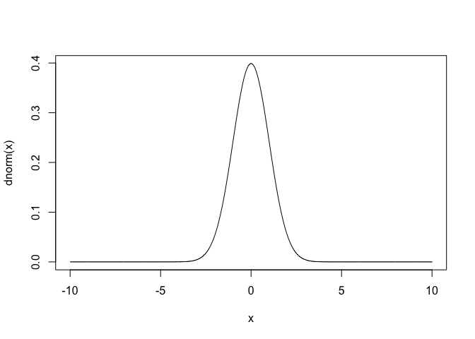
Normal Distribution
\[Normal(\mu, \sigma^{2}): \frac{1}{\sqrt{2\pi}\sigma}e^{-\frac{1}{2}(\frac{x-\mu}{\sigma})^{2}}, -\infty<x<\infty\]x = seq(-10, 10, 0.01)
plot(x, dnorm(x), type="l")
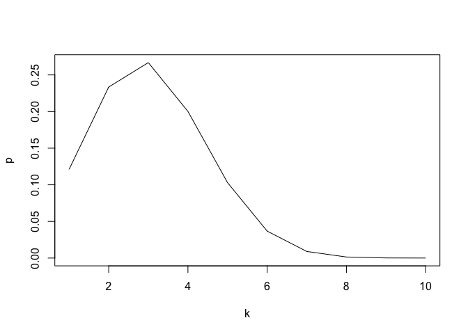
Binomial Distribution
\[Binomial(n,p): \binom{n}{k}p^{k}(1-p)^{n-k}, k=1,2,...,n\]plot(1:10, dbinom(1:10, 10, 0.3), type="l", xlab="k", ylab = "p")
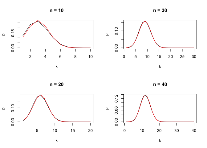
de Moivre - Laplace Theorem
Fix any p strictly between 0 and 1. As the number of trials n increases, the probability histogram for the binomial distribution looks like the nomrla curve with mean np and SD $\sqrt{np(1-p)}$
layout(matrix(1:4,ncol=2))
for(n in 1:4*10){
  plot(1:n, dbinom(1:n, n, 0.3), type="l", main=paste("n = ", n, sep=""), xlab="k", ylab = "p")
  lines(1:n, dnorm(1:n, n*0.3, sqrt(n*0.3*0.7)), col="red")
}
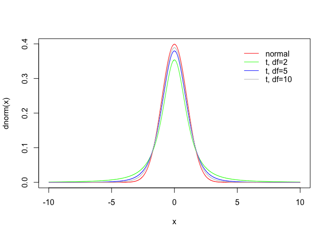
t distribution
With the increase of degree of freedem, t distribution is closer to the standard normal distribution.
x = seq(-10, 10, 0.01)
plot(x, dnorm(x), type="l", col = "red")
lines(x, dt(x, df = 2), col="green")
lines(x, dt(x, df = 5), col="blue")
lines(x, dt(x, df = 10), col="grey")
legend(5,0.40,"normal",lty = 1, col ="red", bty = "n")
legend(5,0.375,"t, df=2",lty = 1, col ="green", bty = "n")
legend(5,0.35,"t, df=5",lty = 1, col ="blue", bty = "n")
legend(5,0.325,"t, df=10",lty = 1, col ="grey", bty = "n")
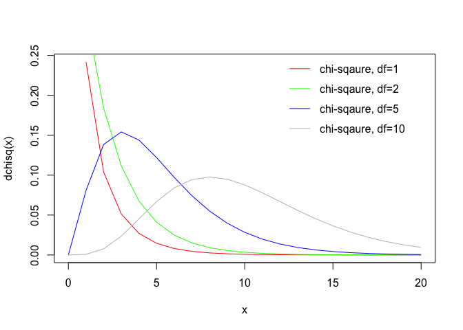
Chi-square distribution
As the degrees of freedom increase, the chi-square curve looks more and more like a normal curve.
x = 0:20
plot(x, dchisq(x, df = 1), type="l", col="red", ylab = "dchisq(x)")
lines(x, dchisq(x, df = 2), col="green")
lines(x, dchisq(x, df = 5), col="blue")
lines(x, dchisq(x, df = 10), col="grey")
legend(12,0.25,"chi-sqaure, df=1",lty = 1, col ="red", bty = "n")
legend(12,0.225,"chi-sqaure, df=2",lty = 1, col ="green", bty = "n")
legend(12,0.2,"chi-sqaure, df=5",lty = 1, col ="blue", bty = "n")
legend(12,0.175,"chi-sqaure, df=10",lty = 1, col ="grey", bty = "n")
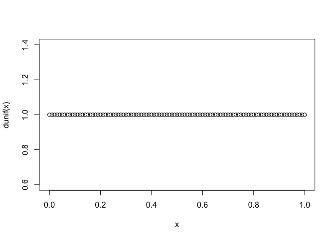
Uniform distribution
\[Uniform(a,b): \frac{1}{b-a}, a \leq x \leq b\]x = seq(0, 1, 0.01)
plot(x, dunif(x))