Statistics Mooc
This is the notebook for Berkley’s Edx course serise - stat2.1, stat2.2, stat2.3.
- Stat2.1 Descriptive Statistics
- Stat2.2 Probability
- Stat2.3 Inference
- Appendix
Stat2.1 Descriptive Statistics
1. Introduction
1.1 Why study descriptive statistics?
- Statistics: The science f drawing conclusions from data
- Descriptive statistics: Describing and summarizing data
- Probability: Understanding and quantifying randomness
-
Inference: Making conclusions based on data from random samples
- Graphical descriptions –> Numerical summaries; single variable –> relation between two variables
1.2 Variables terminology
- quantitative variables
- contiuous and discrete
- categorical and qualitative
1.3 Bar graphs: describing categorical data
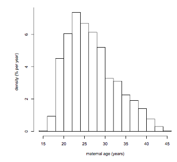
2 The histogram
2.1 Describing one quantitative variable
- Stem and leaf plot
2.2 How to draw a histogram
- show the distribution
- allows for the bariable to be “binned” into unequal intervals
2.3 Units and density
2.4 Percentiles: estimaing from histogram
- famous percentiles
- 25th percentile = lower quartile
- 50th percentile = median
- 75th percentile = upper quartile
2.5 Percentiles: more carefully, from the data
3 Measures of Location
3.1 The median and the mode
- Mode: the value that has the highest frequency
- Unimodal: one peak
3.2 The average: calculation and basic properties
- average/mean: add up all the entries in the list, then divide by the number of entries
- Units of the average: same as the units of the list
3.3 Comparing and combining averages
3.4 The average and the histogram; the average and the median
- The median is unaffected by outliers
- In a right-skewed distribution, the average is greater than the median
3.5 Markov’s inequality
- Markov’s inequality: If a list has only non-negative entries, then the proportion of entries that are >= k times the average is at most $\frac{1}{k}$ (k can be any positive number)
- For example:
- Q: the average age of a group of people is 20 years. What proportion are more than 80 years old?
- A: The proportion is at most $\frac{1}{4}$ (k=4)
4 Measures of spread
4.1 Range and interquartile range
- range = maximum - minimum
- interquartile range (IQR) = upper quartile - lower quartile
- “The IQR of data is 8 years” means “the middle 50% of the data are distributed over 8 years”
4.2 Deviations from average; the standard deviation (SD)
- deviation from average = value - average
- standard deviation (SD) = root mean square (r.m.s.) of deviations from average
- variance = mean sequare of deviations from average
- The average and the SD have the same units
- The vexed question of n-1
In some situations where you are trying to use the SD of a sample to estimate the SD of the population from which the sample was drawn, then according to some criteria, it might be better to use n-1 instead of n in the denominator.
4.3 Properties of the SD; Chebychev’s inequality
- Pafnuty Lvovich Chebychev (1821-1894)
- Chebychev’s inequality: In any list, the proportion of the entries that are k or more SDs away from the average is at most \(\frac{1}{k^{2}}\)
- Rough statement: No matter what the list, the vast majority of entries will be in the range average ± a few SDs
- Precise statment: No matter what the list, a proportion of at least \(1-\frac{1}{k^{2}}\)of the entries will be in the range average ± a few SDs
Typical use

Age: average 20 years, SD 5 years.
What percent are more than 80 years old?

Markov's bound:
at most 25% (1/k, k = 80/20 = 4)

Chebychev's bound:
at most 0.7% (1/k^2, k=(80-20)/5 = 12)

In conclusion, both bounds are correct.
But Chebychev's bound is much sharper.
Because it uses the SD, not just the average.
4.4 Changing units of measurement; standard units
- Mechanics of changing units
- Multiplying by a constant, e.g. centimeters = 2.54 * inches
- Mutliplying by a constant, then adding a constant, e.g. ◦F = (9/5)◦C + 32
- Can also first add a constant, then mulitple by a constant, e.g. new variable = (old variable + b) * a
- Adding a constant
- \[mean_{new} = mean_{old} + constant\]
- \[SD_{new} = SD_{old}\]
- Multiplying by a constant
- \[mean_{mean} = mean_{old} \times constant\]
- \[SD_{new} = SD_{old} * |constant|\]
- Linear transformations: new list = a * (old list) + b
- \[mean_{new} = a \times mean_{old} + b\]
- \[SD_{new} = |a| \times SD_{old}\]
- Standard units: the z-score
- \[z = \frac{x - mean}{SD}\]
- \[x = z \times SD + mean\]
- z measures “how many SDs above mean”
- the mean of any list in standard units is 0
- the SD of any list in standard units is 1
- the vast majority (at least 8/9) of any list in standard units will be in the range -3 to 3
5 The normal curve
5.1 Bell shaped curves; the standard normal curve
- A bell shaped distribution
- The standard normal curve
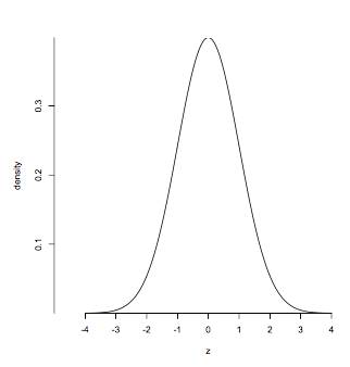
- density at z
Useful to remember

total area = 1
balance point: z=0
points of inflection: z=-1, z=1

Central areas:
between z=-1 and z=1: about 68%
between z=-2 and z=2: about 95%

Tail areas:
to the left of -1: about 16%
to the right of 1: about 16%
to the left of -2: about 2.5%
to the right of 2: about 2.5%

Percentiles:
95th percentils: z=1.65, roughly
5th percentile: z=-1.65, roughly
5.2 Normal curves: relation to the standard normal
-
The normal curve withe mean μ and SD σ
-
density at x
- Finding a percent under a normal curve
For a list with average 67 and SD 3,
what percent are between 63 and 67?

(63-67)/3 = -1.33 standard units
67 = 0 standard units

So, the question becomes:
Under standard normal curve,
what percent are between -1.33 and 0?

The applet says the area is 40.82%.
In R, the expression is "pnorm(0) - pnorm(-1.33)"
5.3 Approximating data histograms; percentiles revisited
5.4 Not all histograms are bell shaped; Chebychev revisited
6 Relation between two variables
6.1 Scatter diagrams
- univariate data: histogram
- bivariate data: scatter diagram
- association: any relation between variables
- positive association
- negative association
- linear association
6.2 The correlation coefficient: calculation and properties
-
correlation coefficient (r): a number between -1 and 1; it measures linear association, that is, how tightly the points are clustered about a straight line
-
If the data are $(x_{i},y_{i}), 1\leq i\leq n$, then
- r is a pure number with no units
- -1 <= r <= 1
- It doesn’t matter if you switch the variables x and y; r stays the same
- Adding a constant to one of the lists, r stays the same
- Multiplying one the lists by a positve constant, r stays the same
- Multiplying just one (not both) of the list by a negative constant, r changes to -r
6.3 Using r: with cation
- Association is not causation
- r measures linear association
- correlated: linearly related
- Even one outlier can have a noticeable effect on r
7 Regression
7.1 Estimation; bivariate normal (“football shaped”) scatter diagrams
- Estimation: one variable, pick one value to estimate.
- natural estimate: the average
- math fact: The r.m.s. of the errors will be smallest if you choose estimator = average.
- average: least squares estimate
- Estimation: two variables, given the value of one variable, estimate the value of the other
- If the scater diagram is roughly football shaped, you can assume:
- the distributions of both the variables are roughly normal
- the distribution of values in each vertical and horizontal strip is roughly normal
- If the scater diagram is roughly football shaped, you can assume:
7.2 Regression line: intuition; the equation in standard units; regression estimates
\[\hat{y} = r \times x, r is the correlation coefficient and x, y in standard units\]7.3 Regression effect, Galton, and the regression fallacy
7.4 Equation of the regression line
the equation in three ways
-
$\hat{y} = r \times x$
-
$ \frac{\hat{y} - \mu_{y}}{\sigma_{y}} = r \times \frac{x - \mu_{x}}{\sigma_{x}}$
-
$\hat{y} = slope \times x + intercept$, where $slope = r \times \frac{\sigma_{y}}{\sigma_{x}}$ and $intercept = \mu_{y} - slope \times \mu_{x}$
8 Error in the regression estimate
8.1 Least squares: why the regression line and no other
- How much error?
- error = vertical distance between the point and the line, for every point in the scatter diagram
- rough size of error = r.m.s of errors
- regreesion line: least squares line
8.2 The r.m.s error of regression; calculations assuming bivariate normal scatter
- r.m.s. error of regression = r.m.s. of residuals = \(\sqrt{1-r^2} \times SD_{y}\)
- r = 1 or -1: r.m.s. error of regression = 0, which says, scatter is a perfect straight line; regression makes no error.
- r = 0: r.m.s. error of regression = SD of y, which says, no linear association; regression is the same as using the average.
- All other r: Regression is not perfect, but better than using the average.
| one variable | two variables |
|---|---|
| normal curve | football shaped scatter diagram |
| average | regression line |
| SD | r.m.s. error of regression |
- Some useful analogies
- For about 68% of the points, the regression estimate of correct to within 1 r.m.s. error.
- For about 95% of the points, the regression estimate is correct to within 2 r.m.s. errors.
- Residual plot
- the average of the residuals is always 0
- there is no linear association between the residuals and x
- the residual plot cannot show any trend or linear relation
- Good regression: residual plot looks like a formless blob around the horizontal axis
8.3 How regression is commonly used; estimating an “unknown true line”
Stat2.2 Probability
1 the two fundamental rules
1.1 What is probability?
- probability of an event = number of outcomes in the event / total number of outcomes
- Frequency theory, long run proportion
- Many probabilities can’t interpreted as long run frequencies, because they are based on experiments that can’t be repeated under identical conditions
1.2 Addition rule
- Probabilities are numbers between 0 and 1
- Notation
- P(A) is read as “the probability that the event A occurs”
- P(A): “probability of A”
- P(coin lands heads), P(heads), P(H)
- Venn diagrams
- Addition rule: P(A or B) = P(A) + P(B), if A and B are mutually exclusive.
- inclusion-exclusion formula: P(A or B) = P(A) + P(B) - P(A and B) for all A and B
- Complement rule: P(not A) = 1 - P(A)
1.3 Multiplication rule
P(B|A): conditional probability of B, given that A has happened- Multiplication Rule:
P(A and B) = P(A) * P(B|A)for all A, B
1.4 Problem-solving techniques
- get started on a solution
- be precise in your use of terminology and notation
- pay attention to detail
- avoid rushing to conclusions
1.5 Conditional or unconditional?
1.6 Bayes’ Rule
P(A) = 0.8; P(B) = 0.2; P(bad|A) = 0.01; P(bad|B) = 0.02

P(A and bad)
 = P(A) * P(bad|A)
 = 0.8 * 0.01
 = 0.008
P(bad)
 = P(A and bad) + P(B and bad)
 = P(A) * P(bad|A) + P(B) * P(bad|B)
 = 0.008 + 0.004
 = 0.012
P(A|bad)
 = P(A and bad) / P(bad)
 = 0.008/0.012
 = 0.67
- Bayes’Rule: Use it to find the conditional probability of an event at an earlier stage, given the result of a later stage.
2 Random sampling with and without replacement
2.1 Independence
- Definition of conditional probability:
P(A and B) = P(A) * P(B|A);P(B|A) = P(A and B)/P(A) - independent trials
- tosses of a coin
- rolls of a die
- draws with replacement
- dependent trials
- cards dealt from a deck
- draws without replacement
- Independent events
- Two events A and B are independent if
P(B|A) = P(B|not A) = P(B) P(A and B) = P(A) * P(B), if A and B are independent
- Two events A and B are independent if
2.2 Sampling with replacement: the binomial formula(二项分布)
- n independent S/F trials (Bernoulli trials)
- p: chance of success on each signle trial
- Bionomial formula
For k = 0,1,2,…,n, the chane of exactly k successes is
\[\binom{n}{k}p^{k}(1-p)^{n-k} = \frac{n!}{k!(n-k)!}p^{k}(1-p)^(n-k)\]2.3 Sampling without replacement: the hypergeometric(超几何) formula
- N: population size
- G: number of good elements in population
- n: simple random sample size
The chance that the sample contains g good elements is
\[\frac{\binom{G}{g}\binom{N-G}{n-g}}{\binom{N}{n}}\]2.4 Examples
- geometric distribution: waiting time till the first sucess; (1-p)k-1*(p) for k = 1, 2, 3…
- negative binomial probabilites
3 the law of averages and expected values
3.1 Not the law of averages
- move from exact calculations to approximations
- Law of averages:
- As you keep tossing, in the long run you get about half heads.
- It is about the proportion of heads being close to 1/2.
3.2 The law of averages
- More formal statment
- As you keep tossing, in the long run, the chance that the proportion of heads is in the range 0.5 ± a fixed amount goes to 1
- You can choose the fixed amount to be as small as you want, as long as you keep it fixed as the number of tosses goes up.
- Law of large numbers
- independent, repeated, success-failur trials
- probability of success on a single trial: p
- As the number of trials increases, the chance that the proportion of successes is in range p ± a fixed amount goes to 1.
3.3 The expected value of a random sum
- Notation:
- random variables: X, Y
- the sum of the first n X’s: Sn = X1 + X2+ … Xn
X: the number of spots on one rool of a die
Probability distribution table for X:
 - spot 1: 1/6
 - spot 2: 1/6
 - spot 3: 1/6
 - spot 4: 1/6
 - spot 5: 1/6
 - spot 6: 1/6

Long run average value of X:
1*1/6 + 2*1/6 + 3*1/6 + 4*1/6 + 5*1/6 + 6*1/6 = 3.5
- Expected value of X = expectation of X = E(X)
- Let X1, X2,…, Xn, be independent and identically distributed (i.i.d.) random variables, and let Sn = X1 + X2+ … Xn. Then, E(Sn) = n*E(X1)
- Exected value of the binomial, E(X) = np
3.4 The expected value of a random average
4 the central limit theorem
4.1 The standard error of a random sum
- Standard error
- The standard error of a random variable X is defined by $SE(X) = \sqrt{E((X-E(X))^{2})}$
- SE(X) measures the rough sie of the chance error in X: roughly how far off X is from E(X)
- Standard deviation
- The standard deviation of a list of numbers: SD = r.m.s. of the deviations from average
- The SD measures the rough size of the deviations: roughly how far off the numbers are from the average
X: one draw at random from 1,2,2,3

X:
P(X = 1) = 1/4
P(X = 2) = 1/2
P(X = 3) = 1/4
E(X) = 2 = average of the box

X-E(X)
P(-1) = 1/4
P(0) = 1/2
P(1) = 1/4
E(X-E(X)) = 0

(X-E(X))^2
P(0) = 1/2
P(1) = 1/2
E((X-E(X))^2) = 0.5

standard error of X = SE(X) = sqrt(E((X-E(X))^2)) = 0.71
= SD of the box (note: for one draw, n = 1)
- n draws at random with replacment from a box of numbered tickets
- average of the box = $\mu$ SD of the box = $\sigma$
Expected value of the sum of draws,
\[E = n\mu\]SE of the sum of draws
\[SE = \sqrt{n}\mu\]4.2 Probabilities for the sum of a large sample
X has the binomial distribution with parameters n and p:
- X is the number of successes in n repeated, independent success-failure trials with probability p of success on a single trial
- X is the sum of n draws with replacement from a 0-1 box that has a proportion p of 1’s
Probability distribution of X:
\[P(\text{X = k}) = \binom{n}{k}p^{k}(1-p)^{n-k}, k=0,1,2,...n\]Expected value of X:
\[E(X) = np\]Standard error of X:
\[SE(X) = \sqrt{np(1-p)}\]- de Moivre - Laplace Theorem
- Fix any p strictly between 0 and 1. As the number of trials n increases, the probability histogram for the binomial distribution looks like the nomrla curve with mean np and SD $\sqrt{np(1-p)}$
4.3 The Central limit theorem
- Central limit theorem
- Rough statment, in English: The probability histogram for the sum of a large number of draws at random with replacement from a box of numbered tickets is approximately normal, regardless of the contents of the box
- Rough statment, in math language: Let X1, X2, …, Xn be independent and identically distributed, each with expected value μ and standard error σ. Let Sn = X1 + X2 + … + Xn. Then for large n, the probability distribution of Sn is approximately normal with mean nμ and SD sqrt(n)σ, no matter what the distribution of each Xi.
4.4 Why you shouldn’t gamble
- Better to use the exact binomial
4.5 The scope of the normal approximation
- It takes lots of draws for the probability histogram for the sum to start looking normal if the contents of the box
- are far from symmetric, for exaple skewed
- have a histogram that has gaps
- Practical advice: Calculate expected value ± 3SE and check whether you are hitting impossible values for the variable
- if you are, the don’t use the normal approximation
- If you are not, then go ahead, but be aware that it still might not be great …
5 the accuracy of simple random samples
5.1 Errors in random percents and averages
- Accuracy of sample average
- population: list of numbers
- n draws at random with replacement from a population that has mean μ and SD σ
- S = sample sum
- E(S) = nμ
- SE(S) = $\sqrt{n}\sigma$
- CLT: If n is large, the distribution of S is roughly normal
- M = sample mean = $\frac{S}{n}$
- E(M) = E($\frac{S}{n}$) = $\frac{n\mu}{n} = \mu$
- SE(M) = SE(S/n) = $\frac{\sqrt{n}\sigma}{n} = \frac{\sigma}{\sqrt{n}}$
- CLT: If n is large, the distribution of M is roughly normal
5.2 Sampling without replacement: the correction factor
- populations: list of N numbers; mean μ and SD σ
- simple ramdom sample of n of these numbers without replacement
- S = sample sum
- E(S) = nμ
- SE(S) = $\sqrt{n}\sigma \times \sqrt{\frac{N-n}{N-1}}$
- M = sample mean
- E(M) = $\mu \times \sqrt{\frac{N-n}{N-1}}$
- $\sqrt{\frac{N-n}{N-1}}$, which is a correction factor (finite population correction), < 1
- When population size N is very large and random sample size n is relatively small, $\sqrt{\frac{N-n}{N-1}}$ ≈ 1, so sampling without replacement is almost the same as sampling with replacement.
Central Limit Theorem (sort of )
Consider a population of size N, with mean μ and SD σ.
Draw a simple random sample of size n.
Then, if n is large in absolute terms but small relative to N:
- the distribution of the sample sum is roughly normal with mean nμ and SE approximately sqrt(n)σ
- the distribution of the sample mean is roughly normal with mean μ and SE approximately σ/sqrt(n)
regardless of the distribution of the population
- Why didn’t we use the correction factor?
- We don’t have the population size, but we know it’s so big that correction factor will be close to 1.
Zeros and ones
- population of G good elements (1’s) and B bad elements (0’s)
- population size N = G + B
- simple random sample size n
- X: number of good elements in sample: hypergeometric N, G, n
- Provided n is small relative to N, it’s same as binomial
- If n is large, but small relative to N, the distribution of X is roughly normal.
5.3 Accuracy
- Square Root law
- If you multiply the sample size by a factor, the accuracy goes up by the square root of the factor
Stat2.3 Inference
1 Estimating unknown parameters
1.1 Random samples
- Terminology
- Population: a collection of units or individuals
- Parameter: a number associated with the population
- Sample: a subset of the population
- Estimate: a number computed from the sample, and used as a guess for the parameter
- Try to avoid or reduce bias in the sample
- Selection bias
- Non-response bias
- Bigger isn’t always better. If the method of sampling is bad, taking a large sample doesn’t help. You just get a big bad sample.
- Random sample or probability sample: Before the sample is drawn, it has to be possible to calculate the probability (doesn’t have to be the same) with each member of the population will be included in the sample.
- Types of samples
- sample of convenience, not a random sample
- simple random sample: draws uniformly at random without replacement from the population; random sample
- Cluster sample: random smaple
1.2 Estimating population averages and percents
- Sampling assumption: Simple random sample; large, but still small relative to the population, so that the correction factor is almost 1.
- Bootstrap method - use sample SD as an approximation to population SD
1.3 Approximate confidence intervals
- sampling assumptions:
- simple random sample
- large enough so that the probability histogram for the sample mean or sample percent is roughly normal by Central Limit Theorem
- but small enough relative to the population size that the correction factor is close to 1
- confidence intervals: sample mean ± 2 * SE of sample mean
1.4 Interpreting confidence intervals
2 Testing Statistical Hypotheses
2.1 Testing hypotheses: terminology
- Terminology and method
- null hypothesis: H0
- alternative hypothesis: H1
- Assuming the null is true, the chance of getting data like the data in the sample or even more like the alternative: P-value
- Methods: If P is small, choose the altrnative. Otherwise, stay with the null
- Conventional definition:
- “small”: P<5%, the result is statistically significant
- “very small”: P<1%, the result is highly statistically significant
2.2 Tests for a population proportion
- Testing for a binomial p
Genetic theory: each plant has a 25% chance of being red-flowering.
Experiment data: 400 plants of this species; 88 are red-flowering
Question: Is the theory good, or are ther two few red?
Answer:
n=400; H0:p=0.25; H1:p<0.25

exact binomial test:
P(k<=88)=9.08%

one-sample z test:
approximately normal with mean 100 (400*0.25) and SD 8.66(sqrt(400*0.25*0.75))
z = (88.5 - 100)/8.66 = -1.328
P-value = 9.21%
2.3 Significance level and P-value
- H0: p = 0.5
- H1: p = 0.8
- experiments: coin will be tossed 20 times
- test: if the number of heads is 14 or more, choose H1; otherwise choose H0
| test concludes: p=0.5(Not Reject H0) | test concludes: p=0.8(Reject H0) | |
|---|---|---|
| reality is 0.5 (H0 is true) |
correct conclusion | type I error Probability: binomial, n=20, p=0.5, P(k>=14)=5.8% significance level |
| reality is 0.8 (H0 is false) |
type II error | correct conclusion Probability: binomial, n=20, p=0.8, P(k>=14)=91.3% power |
- Two criteria for a good test
- significance level = probability, under H0, that the test concludes H1 error probabilty, should be small
- power = Probability, under H1, that the test concludes H1 probability of correct conclusion, should be large
2.4 One tail or two?
3 One-sample and two-sample tests
3.1 z-test for a population mean
- H0: μ = 69.5
- H1: μ < 69.5
- SRS: n=100, mean=69, sd=2.5
- If the null were true,
- expectd value of sample mean = 69.5
- SE of sample mean = population SD / sqrt(n) ≈ sample SD / sqrt(n) = 0.25
- z = (69-69.5)/0.25 = -2, P ≈ 2.5%
- Conclustion: Reject the null; μ < 69.5
3.2 t-test for a population mean
- H0: μ = 30
- H1: μ > 30
- SRS: n=5, mean=31.56 (31.8, 30.9, 34.2, 32.1, 28.8)
Sample is small; can’t apply Central Limit Theorem to the distribution fo the sample mean; can’t assume the probabilities for sample mean are normal.
- If the null were true,
- expected value of sample mean = 30
- SE of sample mean = ??/sqrt(5)
How to approximate ?? based on such a small sample?
- Better estimate of unknown σ is a bit bigger
- SD of sample * sqrt(n/n-1)
- SE of sample mean = 1.94604/sqrt(5) = 0.877
- t = (31.56-30)/0.877 = 1.79
t distribution
- close relative of z
- there are many t curves, one for each sample size
- degrees of freedom = n -1
- P = 7.2% > 5%
- Conclusion: Don’t reject null; belief that population mean = 30 isn’t bad
One-sample t test: summary of method
- Test for a population mean (unknown SD); sample size n
- One-sample t test is just like one-sample z test for population mean
- Same null and alternative hypotheses, same calculation, except:
- Assume population distribution roughly normal, unknown mean and SD
- Approximate unknown SD of population by sample SD, with n-1 in the denominator
- Use t curve, degrees of freedom = n-1
3.3 Testing for the difference between means
- SE of the difference between independent random variables: SE(X-Y) = sqrt(Var(X) + Var(Y))
SRS1(e.g. average household income in City A): n=200, mean=518, SD=100
SRS2(e.g. average household income in City B): n=250, mean=509, SD=110
H0: μ1 = μ2
H1: μ1 > μ2

If the null were true,
expected difference between the sample means would be 0,
with an SE of approximately:
SE = sqrt(SE1^2 + SE2^2) = sqrt((SD1/sqrt(n1))^2 + (SD2/sqrt(n2))^2) = 9.92

But observed difference between the sample means is 9,
z = (9-0)/9.92 = 0.907
the P-value is 18.2%

Conclusion: Stay with the null; the difference just looks like chance variation.
3.4 Testing for the difference between proportions
SRS1: n=500, proportion=34%
SRS2: n=750, proportion=40%
H0: p1 = p2
H1: p1 < p2

Observed difference in sample percents: 6%

If the null is true,
expected difference in sample percents is 0,
both sample are from a population with a propotion
phat = (p1 * n1) + (p2 * n2) = 0.376
SE1 ≈ sqrt(phat*(1-phat)/n1) = 0.022
SE2 ≈ sqrt(phat*(1-phat)/n2) = 0.018
SE of the difference between the sample percents is approximately
sqrt(SE1^2 + SE2^2) = 2.8%
z = (6%-0)/2.8% = 2.14
p-value ≈ 1.6%

Conclusion: Alternative
4 Dependent Samples
4.1 Paired samples: parametric analysis
SRS(e.g. students): n=100
measure1(e.g. math score): mean=68, SD=12
measure2(e.g. verbal score): mean=72, SD=14
H0: md = 0 (md = measure1 - measure2)
H1: md != 0

Observed md: -4

If the null is ture,
expected md is 0,
the SE ???

Caclulate the SD of md in SRS = 11.76
OR
SD = sqrt(var(x) + var(y) - 2Cov(x,y)) = 11.76
(because x, y are not independent)

SE = 11.76/sqrt(100) = 1.176
z = (-4 - 0)/1.176 = -3.4
P is tiny

Conclusion: Reject the null
4.2 Paired samples: non-parametric analysis
SRS(e.g. students): n=100
measure1(e.g. math score): mean=68, SD=12
measure2(e.g. verbal score): mean=72, SD=14
H0: md = 0 (md = measure1 - measure2)
H1: md != 0

Calculate the number (e.g. 62) of measure1 - measure2 < 0
p = binomial(k>=62, n, 0.5) = 1.05%

Conclusion: md < 0
- The calculation ignores much of the information in the scores
- Difference di = xi-yi is math - varbal for Student i. Test just used the number of differences that were negative.
- Throws away the scores (apart from these signs), so can be quite rough
- But easier to carry out than our previous method, and requires no additional assumptions when the sample is small.
4.3 Randomized experiments: method
A sample of randomized controlled experiments
- experiment to test effectiveness of "cheat sheets" on probability exame
- 300 students agree to participate in a study
- Treatment group: SRS of 200 is allowed to bring cheat-sheet into the exam.
- Control group: The remaining 100 take the exam without the cheat-sheet.
- Data:
	- Treatment group: mean=75, SD=15
	- Control group: mean=80, SD=12

- Did the treatment hurt?
- Method: use the two-sample z test.
4.4 Randomized experiments: justification
- Dubious step 1:
1/sqrt(200) = 1.06, 12/sqrt(100)=1.2- Missing the correction factor. The correction factor cannot be ignored due to the raito of sample size (100 or 200) and population size (300)
- Theses results are bigger than they should be
- Dubious step 2:
sqrt(1.06^2 + 1.2^2)- Pretends that treatment and control groups are independent.
- sqrt(a^2+b^2) produces a result that is smaller than it should be.
- The two errors offset each other. The result is a slight overestimate of SE, close to correct.
5 Window to a wider world
5.1 Not everything’s normal: chi-squared test
A categorical data: more than two categories
Sample of students at a large university:
	- 54 freshmen
	- 40 sophomores
	- 51 juniors
	- 39 seniors
	- 16 graduate
H0: The data are lkie a simple random sample from a large population consisting of 22.5% each of freshmen, sophomores, juniors, and seniors, and 10% graduate students.
H1: The data are not like a simple random sample from the population in the null.
- Compare the observed counts to what the null predicts:
| F | So | J | Se | G | Total | |
|---|---|---|---|---|---|---|
| observed | 54 | 40 | 51 | 39 | 16 | 200 |
| expected, under null | 45 | 45 | 45 | 45 | 20 | 200 |
| o-e | 9 | -5 | 6 | -6 | -4 | 0 |
| (o-e)^2/e | 1.8 | 0.556 | 0.8 | 0.8 | 0.8 | 4.756 |
Test statistic = $\displaystyle\sum{\frac{(o - e)^2}{e}}$ over all categories ~ chi-square(X2) distribution, with degrees of freedom = number of categories - 1
- Facts about chi-square distributions
- Values are non-negative
- expected value = balance point = degrees of freedom
- SD = sqrt(2 * degrees of freedom)
- As the degrees of freedom increase, the chi-square curve looks more and more like a normal curve.
x = matrix(c(54, 40, 51, 39, 16, 45, 45, 45, 45, 20), nrow=2, byrow=T)
chisq.test(x[1,], p=x[2,]/sum(x[2,]), correct=F)
5.2 How Fisher used the chi-squared test
- Test raises questions about the accuracy of Mendel’s data: the deviations from his models were smaller than would be expected by chance.
5.3 Chi-squared test for independence
- SRS of students at a large university
Observed result
| female | male | total | |
|---|---|---|---|
| delared science | 62 | 21 | 83 |
| declared other | 137 | 74 | 211 |
| undeclared | 48 | 58 | 106 |
| total | 247 | 153 | 400 |
- Question: At the university, are gender and major declaration status independent?
- H0: independent; H1: not independent
Expected result: $\text{expected count} \approx \frac{\text{row total} \times \text{column total}}{\text{grand total}}$
| female | male | total | |
|---|---|---|---|
| delared science | 51.25 | 31.75 | 83 |
| declared other | 130.29 | 80.71 | 211 |
| undeclared | 65.45 | 40.55 | 106 |
| total | 247 | 153 | 400 |
- Add $\frac{(o-e)^{2}}{e}$ over all 3 * 2 cells
- $\chi^{2} \text{statistic} \approx 19$
- degrees of freedom = (rows - 1) $\times$ (columns -1) = (3-1)$\times$(2-1) =2
- p = 7.485183e-05, tiny
- Conclusion: Not independent
Appendix
Appendix 1 : The Greek Symbols
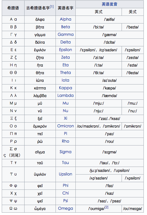
source: https://zh.wikipedia.org/wiki/%E5%B8%8C%E8%85%8A%E5%AD%97%E6%AF%8D
Appendix 2 : Common Distribution
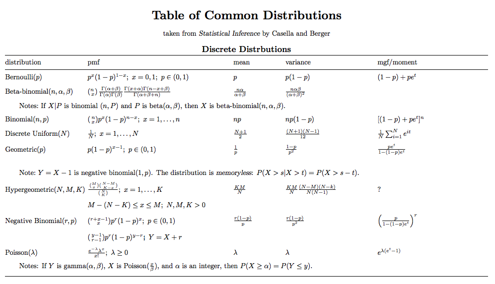
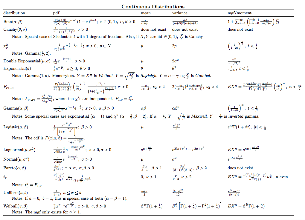
ps: pmf, probability mass function(概率质量函数); pdf, probability density function(概率密度函数); mgf, Moment-generating function(动差生成函数)
source: http://www.stat.tamu.edu/~twehrly/611/distab.pdf
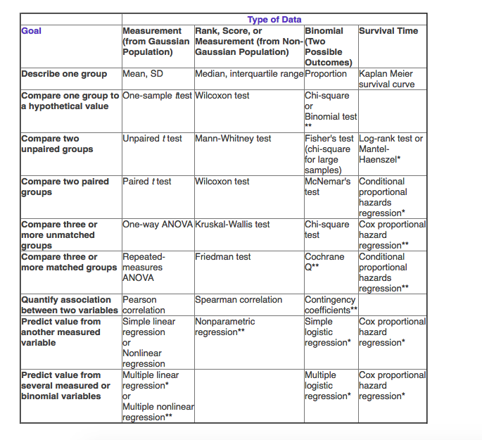
Appendix 3: how to choose statistical test